Let's Learn Excel
-
Professional Development CoursesLet's Learn ExcelResume0% complete0% complete
Introduction
-
Students mustStudent must submit this questionnaire to complete it
Show More-
Welcome to our comprehensive Excel course designed to equip you with essential skills for mastering this powerful spreadsheet software. Throughout this course, you will embark on a journey from Excel novice to proficient user, gaining a deep understanding of its features and functionalities. Whether you're a beginner seeking to grasp the basics or a seasoned user aiming to enhance your proficiency, this course offers a structured learning path to cater to your needs.


There are four (4) modules in this course :
- "Introduction to Excel" lays the foundation by covering core concepts like spreadsheets, workbooks, and worksheets.
- "Calculations and Functions" focuses on mastering basic arithmetic operations, cell referencing, and utilizing Excel's built-in functions.
- "Excel Charts" explores data visualization techniques, including creating various types of charts to effectively present data.
- "A Closer Look At Working with Excel Cells" delves into advanced techniques such as cell referencing, sorting, and filtering for precise data manipulation.
This course has a total completion time of
Let's Learn Excel was developed by Dr. Marco Aurelio Hernandez; Ph.D.(Biostatistics); MSc (Stat); MSc (Edu); BSc (Biology).Engaging with this course
To register for this course, complete the registration form. Begin the course with Module 1. For each lesson, read the description.
You can click on the collection of resources in each module.
There is a forum in each Module for activity submission and peer evaluation, and you can add a new topic or respond to a previous one. You can share your learning from this and other readings, comment on the topics from your own experience, comment on others' posts, or provide feedback on how we can improve the content and/or presentation.
Requirements to obtain the certificate
You may browse this course for free to learn for your personal enrichment. There are no requirements.
To obtain a certificate, a learner must successfully complete:
- All reading requirements
- All activities
- The self and course evaluation forms
-

Covered in this module:
In this module, you will grasp the fundamentals of Excel, including understanding spreadsheets, workbooks, and worksheets. You will focus on identifying and utilizing different parts of an Excel worksheet while also learning essential data entry techniques and basic formatting skills for fonts, alignment, and numbers.
-
Student Learning Outcomes:
Upon completion of this lesson, you will be able to:
- knowledgeably discuss what Excel is, as well as spreadsheets, workbooks, and some main aspects of worksheets.
- Point out the parts of an Excel worksheet and give their functions.
-
Required Learning Resources and Activities
-
-
Students mustMark as done
Watch the entire video. (12 minutes)
48.6 MB
-
Student Learning Outcomes:
Upon completion of this lesson, you will be able to:
- Correctly enter data into a table in the worksheet.
-
Required Learning Resources and Activities
-
Students mustView
Watch the entire video. (20 minutes)
92.7 MB -
Students mustMark as done
Do the hands-on exercise. (30 minutes)
314.2 KB -
-
Students mustView
Do the hands-on exercise. (30 minutes)
449.5 KB -
-
Student Learning Outcomes:
Upon completion of this lesson, you will be able to:
- Format the font family, size, color, alignment and numbers in a worksheet.
-

Students mustMark as done
Required Learning Resources and Activities
-
-
Students mustMark as done
Watch the entire video. (14 minutes)
200.3 MB -
-
-

Covered in this module:
Here, you'll delve into the realm of calculations and functions in Excel, mastering basic arithmetic operations and leveraging cell referencing effectively. You'll explore the power of Excel's autofill feature for generating series, lists, and formulas efficiently. Moreover, you'll gain proficiency in utilizing Excel's built-in functions to streamline calculations and other operations.
-
Student Learning Outcomes:
Upon completion of this lesson, you will be able to:
- Perform basic calculations like addition, subtraction, multiplication, division, powers, and roots with Excel.
- Use cell referencing in calculations.
-
Required Learning Resources and Activities
-
-
Student Learning Outcomes:
Upon completion of this lesson, you will be able to:
- Perform calculations using Excel autofill for series, lists, and formulas.
- Use autofill.
-
Students mustMark as done
Required Learning Resources and Activities
-
-
-
Student Learning Outcomes:
Upon completion of this lesson, you will be able to:
- Use Excel's built-in functions for calculations and other operations.
- Use formulas and functions.
-

Students mustMark as done
Required Learning Resources and Activities
-
-
-
-
-
-
Students mustViewMake a submission
Activity 1, Module 2. (30 minutes)
Calculations
Instructions
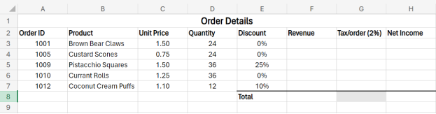
You are given the order details of a bakery in the table below. Complete the activity by following the instructions.
1. Open Excel and create the table given in an Excel worksheet

2. Calculate the revenue and tax on the revenue for each of the five products.
3. Calculate the net income of each product.
4. Calculate the total revenue from all products.
5. Calculate the total net income of all products. -
Students mustViewMake a submission
Activity 2, Module 2 (30 minutes)
Formulas and Functions
Instructions
Download the dataset “Activity_Module2_Worksheet.xlxs.” Complete the activity by following the instructions below.
1. Open the file “Activity_Module2_Worksheet.xlxs.”
2. Create a formula that calculates the gross pay for each employee, then use a built-in function to calculate the total gross pay. The gross pay total should appear in cell “E14.” All totals should appear in Row 14.
3. Create a formula that calculates the tax, which is 20% of the gross pay for each employee, then calculate a total for the tax.
4. Create a formula that calculates the net pay for each employee, then calculate a total for the net pay.
5. Create a formula that calculates the superannuation, which is 8% of the gross pay for each employee, then calculate a total for the superannuation. 6. Use functions to determine the average, maximum, and minimum values for each column, setting the number of decimal places to 2. The average, maximum, and minimum values for each column should appear in Rows 16, 17, and 18, respectively.
7. Use the “Save As” command to save the workbook as “Activity Formulas and Functions (Completed).xlxs.”
-

Covered in this module:
This module focuses on visualizing data effectively through charts in Excel. You'll learn to create basic charts, pie charts, bar charts, as well as single- and multiple-series scatterplots and line charts. By the end, you'll be equipped with the skills to present data graphically for clearer insights.
-
Student Learning Outcomes:
Upon completion of this lesson, you will be able to:
- Create basic charts and pie and bar charts to visualize your data.
-
Required Learning Resources and Activities
-
-
-
Students mustViewMake a submission
Activity 1, Module 3: Basic Charts (30 minutes)
Part 1
1. Open Excel.
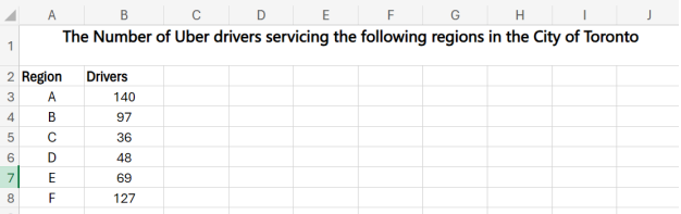
2. Enter the data into your spreadsheet, as shown in the figure below.
3. Use the given data to create a pie chart.
4. Make the chart a large size for ease of use.
5. Give the chart the title “The Number of Uber Drivers ServicingRegions A – F for March 2024.”
6. Move the legend to the right of the plot area.
7. Change the values to percentages and move the pie labels to the outside of the pie slices.
-
Student Learning Outcomes:
Upon completion of this lesson, you will be able to:
- Create single- and multiple-series scatterplots and line charts.
-

Students mustMark as done
Required Learning Resources and Activities
-
-
Students mustViewMake a submission
Activity 2, Module 3: Scatterplots and Line Graphs (30 minutes)
Part 1: Scatterplots
1. Open Excel.
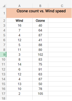
2. Enter the data into your spreadsheet, as shown in the figure below.
3. Use the given data to create a scatterplot. When selecting the data, do not include the merged cells A1 – C1.
4. Make the chart a large size for ease of use.
5. Give the chart the title “Wind Speed vs. Ozone Level in the Northern Region.”
6. Shade the background of the merged cells in a color of your preference.
7. Change the color of the dots to your preference by pointing the cursor at one of the dots, right-clicking, choosing “Format > Fill,” and selecting the color you want.Part 2: Line Graphs
1. Open Excel.
2. Open the dataset for the exercise “Dataset_Exercise2_Module3.xlxs.”
3. We are going to plot the line chart for all fruits for the month of January.
4. Select the range A2 to F3.
5. Get the line chart by going to “Insert,” then “Charts,” then “Line Chart,” with the first option of the smooth line or the option with the line plus the nodes. This is the line chart for January sales. Label it appropriately.
6. Now, we are going to make a line chart with the sales for all months of the year.
7. Select the range A2 to F12.
8. Go to “Insert,” then “Charts,” then “Line Chart.” Choose the option with the nodes to visualize the individual month lines more clearly.
9. This should give you a chart with 12 lines, one for the sales of fruit for each month.
10. Label the chart appropriately
-
Covered in this module:In this module, you'll delve deeper into working with cells in Excel, mastering techniques like relative and absolute referencing in calculations and formulas. You'll also learn advanced data manipulation skills such as sorting and custom-sorting sheets and ranges, as well as filtering and custom-filtering datasets for more refined analysis.
-
Student Learning Outcomes:
Upon completion of this lesson, you will be able to:
- Use relative and absolute referencing in calculations and formulas.
-
Required Learning Resources and Activities
-
Students mustView
Read the entire article. (10 minutes)
1.7 MB -
-
Students mustViewMake a submission
Activity 1, Module 4: Relative and Absolute Referencing (30 minutes)
1. Open Excel.
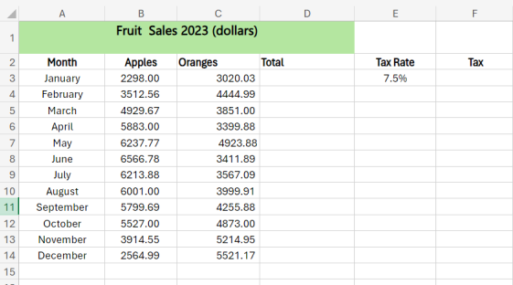
2. Enter the data into your spreadsheet, as shown in the figure below.
3. In cell D3, enter the formula that calculates the total sales for the month of January.
4. Copy the formula down to column D for all other months of the year by dragging the fill handle or double-clicking.
5. Click on cell E3. Click on the down arrow in the “Number” section of the “Home” tab. Proceed to the panel on the right, and make sure you have 1 decimal place.
6. In cell F3, enter the formula that calculates the tax on the total sales for the month. The tax rate is 7.5%. This is where you use absolute referencing. 7. By dragging the fill handle or double-clicking, copy the formula down to column F for all other months of the year.
8. Type “TOTAL” in cell C15.
9. Using the SUM function, find the total sales for the year and the total tax paid. Total sales will go into cell D15, and the total tax will go into cell F15.
-
Student Learning Outcomes:
Upon completion of this lesson, you will be able to:
- Sort and custom-sort a sheet and a range with the sort function.
-
Students mustMark as done
Required Learning Resources and Activities
-
-
-
-
Students mustViewMake a submission
Activity 2, Module 4: Sorting (30 minutes)
1. Open the workbook with the dataset for Activity 2, Module 4: Dataset_Activity2_Mod4.xlxs.
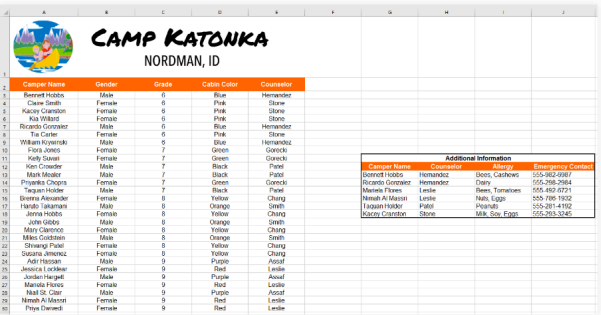
2. For the main table, create a custom sort that sorts by grade from smallest to largest and then by camper name from A to Z.
3. Create a sort for the additional information section. Sort by counselor (column H) from A to Z.
When you’re finished, your workbook should look like this:
-
-
-
Students mustViewMake a submission
Do the hands-on activity- 30 minutes
-
-
Student Learning Outcomes:
Upon completion of this lesson, you will be able to:
- Filter and custom-filter a sheet dataset with the filter commands.
-

Students mustMark as done
Required Learning Resources and Activities
-
-
-
Students mustViewMake a submission
Activity 3, Module 4: Filtering Basics
1. Open the workbook with the dataset for Activity 3, Module 4: Dataset_Activity3_Mod4.xlxs.
2. Apply a filter to show only electronics and instruments.
3. Clear that Filter.
4. Using a number filter, show loan amounts greater than or equal to $100. 5. Filter the resulting dataset to show only items that have deadlines in 2016 -
-
-
-
In this section, you can provide feedback about this course to help us make NextGenU.org better. Once evaluations are completed, you will be able to download your certificate of completion.Not available unless: The activity Course Registration is marked complete ...Not available unless:- The activity Course Registration is marked complete
- The activity Activity 1, Module 3 is marked complete
- The activity Activity 1, Module 2 - Calculations is marked complete
- The activity Activity 2, Module 2 - Formulas and Functions is marked complete
- The activity Activity 2, Module 3 is marked complete
- The activity Activity 1, Module 4 is marked complete
- The activity Activity 2, Module 4 - Custom Sorting is marked complete
- The activity Activity 3, Module 4 - Filtering Basics is marked complete
-
Course Evaluation QuestionnaireNot available unless: The activity Course Registration is marked complete
-
Self Evaluation QuestionnaireNot available unless: The activity Course Registration is marked complete
-
-
Students mustMark as done
-
-